こんにちは!ぼりたそです!
今回はを使用して獲得関数による探索効率にどのような影響があるかを検証してみました。
以前まとめたベイズ最適化の実装についての記事も合わせて参考にしてみてください。

この記事は以下のポイントでまとめています。
- ベイズ最適化のフロー
- ベイズ最適化条件
- ベイズ最適化の結果
結論から言うと、今回実行したベイズ最適化のデータセットにおいてはカーネルの種類によって探索効率に違いが出ました。
当たり前かもしれませんが、カーネルの選択は大事なんだなあと実感する結果でした。
ちなみに、今回のデータセットは以前PubChemから取得した化合物のXlogP(目的変数)とmordred記述子(説明変数)を使用しています。
今回使用したデータは以下からダウンロードできます。data_yが目的変数、data_xが説明変数となっています。
※CSVではアクセスできないようなので、エクセルファイル(.xlsx)をダウンロードしてCSVとしてエクスポートしていただけますと使用できるかと思います。
それでは以下、詳細について説明していきます。
ベイズ最適化のフロー
まず、今回のベイズ最適のフローについて以下のフローチャートにて示します。
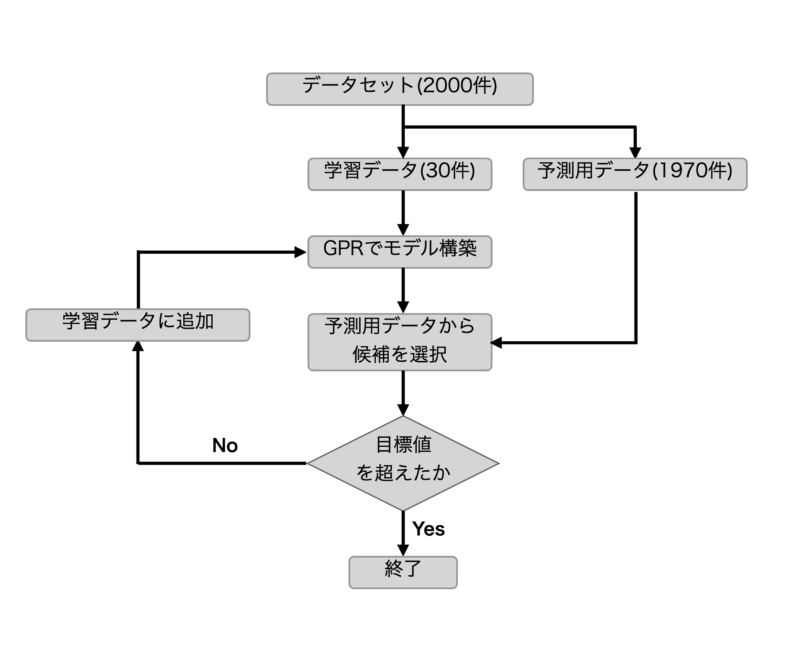
フローとしてはまず、データセットを学習用データ30件、予測用データ1970件に分割します。
その後、学習用データからGPR(ガウス過程回帰)で学習モデルを構築します。
学習モデルから予測用データの中から次の候補を選択します。
候補の値が目標値を越えれば終了、越えていなければ候補点を学習用データに加えて再度学習モデルを構築する。
以上の流れで最適化をおこなっています。
また、目標値に関しては予測用データの最大値(XlogP=22.4)を設定しています。
ベイズ最適化の条件
次に今回行ったベイズ最適化の条件を説明していきます。
具体的な条件は以下の通りです。
■目的 カーネルによって最適化効率にどのような影響があるかを確認
■検討カーネル 11種(明治大学 金子弘昌先生のコード参照)
■目的関数 XlogP
■説明変数 Mordred記述子(916個)
■獲得関数 EI
■最適化目標値 予測用データの最大値(22.4)
また、下に今回使用したコードを示します。今回使用したコードは明治大学 金子弘昌先生がGithubにて公開されているものを参考にしています。
金子弘昌先生が公開しているコード↓↓↓↓↓
https://github.com/hkaneko1985/python_doe_kspub/blob/master/sample_program_05_04_bayesian_optimization.py
まずはデータセットを学習用データと予測用データに分割して保存するコードです。こちらは自分で記述しました。
#データセット約2000件を学習用データ、予測用データに分割して保存。
#seed値を0〜90として10セット生成
import pandas as pd
import random

# CSVファイルの読み込み
data_x = pd.read_csv('data_x.csv', index_col='cid')
data_y = pd.read_csv('data_y.csv', index_col='cid')

# 抽出する行数が元の行数より多い場合は、元の行数に合わせる
num_rows = min(30, len(data_x))

#Seed値を設定
seed = [x for x in range(0,91) if x%10==0]

for seed in seed:
    # ランダムに行を抽出
    random_rows = data_x.sample(n=num_rows, random_state=random.seed(seed))

    # 抽出した行を別のファイルに保存する場合
    random_rows.to_csv(f'train_x_seed_{seed}.csv', index='cid')
    data_y.loc[random_rows.index].to_csv(f'train_y_seed_{seed}.csv', index='cid')

    # 元のデータから抽出した行を削除
    data_x = data_x.drop(random_rows.index)
    data_y = data_y.drop(random_rows.index)

    # 更新されたデータを別のファイルに保存する場合
    data_x.to_csv(f'prediction_data_x_seed_{seed}.csv', index='cid')
    data_y.to_csv(f'prediction_data_y_seed_{seed}.csv', index='cid')
次にベイズ最適化のコードです。金子弘昌先生が記述子したコードに少し手を加えています。(金子先生、完璧なコードに傷をつけてしまいすみません…)
###### -*- coding: utf-8 -*-
"""
@author: Hiromasa Kaneko
"""

import pickle
import matplotlib.pyplot as plt
import pandas as pd
import numpy as np
from scipy.stats import norm
from sklearn.model_selection import KFold, cross_val_predict
from sklearn.gaussian_process import GaussianProcessRegressor
from sklearn.gaussian_process.kernels import WhiteKernel, RBF, ConstantKernel, Matern, DotProduct
from sklearn.metrics import r2_score, mean_squared_error, mean_absolute_error

regression_method = 'gpr_one_kernel'  # gpr_one_kernel', 'gpr_kernels'
acquisition_function = 'EI'  # 'PTR', 'PI', 'EI', 'MI'

fold_number = 10  # クロスバリデーションの fold 数
kernel_number = 3  # 0, 1, 2, 3, 4, 5, 6, 7, 8, 9, 10
target_range = [0, 1]  # PTR
relaxation = 0.01  # EI, PI
delta = 10 ** -6  # MI


#seed値の設定
seed = [x for x in range(0,91) if x%10==0]

for seed in seed:

    suggest_data = []
    suggest_xlogp = 0
    trial = 0

    #dataset = pd.read_csv('resin.csv', index_col=0, header=0)
    x_prediction = pd.read_csv(f'prediction_data_x_seed_{seed}.csv', index_col=0, header=0)
    y_answer = pd.read_csv(f'prediction_data_y_seed_{seed}.csv', index_col=0, header=0)

    # データ分割
    y = pd.read_csv(f'train_y_seed_{seed}.csv', index_col=0, header=0)  # 目的変数
    y = y.iloc[:,0]
    x = pd.read_csv(f'train_x_seed_{seed}.csv', index_col=0, header=0)  # 説明変数

    # 標準偏差が 0 の特徴量の削除
    deleting_variables = x.columns[x.std() == 0]
    x = x.drop(deleting_variables, axis=1)
    x_prediction = x_prediction.drop(deleting_variables, axis=1)

    # カーネル 11 種類
    kernels = [ConstantKernel() * DotProduct() + WhiteKernel(),
               ConstantKernel() * RBF() + WhiteKernel(),
               ConstantKernel() * RBF() + WhiteKernel() + ConstantKernel() * DotProduct(),
               ConstantKernel() * RBF(np.ones(x.shape[1])) + WhiteKernel(),
               ConstantKernel() * RBF(np.ones(x.shape[1])) + WhiteKernel() + ConstantKernel() * DotProduct(),
               ConstantKernel() * Matern(nu=1.5) + WhiteKernel(),
               ConstantKernel() * Matern(nu=1.5) + WhiteKernel() + ConstantKernel() * DotProduct(),
               ConstantKernel() * Matern(nu=0.5) + WhiteKernel(),
               ConstantKernel() * Matern(nu=0.5) + WhiteKernel() + ConstantKernel() * DotProduct(),
               ConstantKernel() * Matern(nu=2.5) + WhiteKernel(),
               ConstantKernel() * Matern(nu=2.5) + WhiteKernel() + ConstantKernel() * DotProduct()]


    while suggest_xlogp != 22.4:

        trial += 1
        print(f'trial:{trial}')

        # オートスケーリング
        autoscaled_y = (y - y.mean()) / y.std()
        autoscaled_x = (x - x.mean()) / x.std()
        autoscaled_x_prediction = (x_prediction - x.mean()) / x.std()

        print(f'目標値:XlogP=22.4')

        # モデル構築
        if regression_method == 'gpr_one_kernel':
            selected_kernel = kernels[kernel_number]
            model = GaussianProcessRegressor(alpha=0, kernel=selected_kernel)
        elif regression_method == 'gpr_kernels':
            # クロスバリデーションによるカーネル関数の最適化
            cross_validation = KFold(n_splits=fold_number, random_state=9, shuffle=True) # クロスバリデーションの分割の設定
            r2cvs = [] # 空の list。カーネル関数ごとに、クロスバリデーション後の r2 を入れていきます
            for index, kernel in enumerate(kernels):
                print(index + 1, '/', len(kernels))
                model = GaussianProcessRegressor(alpha=0, kernel=kernel)
                estimated_y_in_cv = np.ndarray.flatten(cross_val_predict(model, autoscaled_x, autoscaled_y, cv=cross_validation))
                estimated_y_in_cv = estimated_y_in_cv * y.std(ddof=1) + y.mean()
                r2cvs.append(r2_score(y, estimated_y_in_cv))
            optimal_kernel_number = np.where(r2cvs == np.max(r2cvs))[0][0]  # クロスバリデーション後の r2 が最も大きいカーネル関数の番号
            optimal_kernel = kernels[optimal_kernel_number]  # クロスバリデーション後の r2 が最も大きいカーネル関数
            print('クロスバリデーションで選択されたカーネル関数の番号 :', optimal_kernel_number)
            print('クロスバリデーションで選択されたカーネル関数 :', optimal_kernel)

            # モデル構築
            model = GaussianProcessRegressor(alpha=0, kernel=optimal_kernel) # GPR モデルの宣言

        model.fit(autoscaled_x, autoscaled_y)  # モデル構築

        # トレーニングデータの推定
        autoscaled_estimated_y, autoscaled_estimated_y_std = model.predict(autoscaled_x, return_std=True)  # y の推定
        estimated_y = autoscaled_estimated_y * y.std() + y.mean()  # スケールをもとに戻す
        estimated_y_std = autoscaled_estimated_y_std * y.std()  # スケールをもとに戻す
        estimated_y = pd.DataFrame(estimated_y, index=x.index, columns=['estimated_y'])
        estimated_y_std = pd.DataFrame(estimated_y_std, index=x.index, columns=['std_of_estimated_y'])


        # トレーニングデータの実測値 vs. 推定値のプロット
        plt.rcParams['font.size'] = 18
        plt.scatter(y, estimated_y.iloc[:, 0], c='blue')  # 実測値 vs. 推定値プロット
        y_max = max(y.max(), estimated_y.iloc[:, 0].max())  # 実測値の最大値と、推定値の最大値の中で、より大きい値を取得
        y_min = min(y.min(), estimated_y.iloc[:, 0].min())  # 実測値の最小値と、推定値の最小値の中で、より小さい値を取得
        plt.plot([y_min - 0.05 * (y_max - y_min), y_max + 0.05 * (y_max - y_min)],
                 [y_min - 0.05 * (y_max - y_min), y_max + 0.05 * (y_max - y_min)], 'k-')  # 取得した最小値-5%から最大値+5%まで、対角線を作成
        plt.ylim(y_min - 0.05 * (y_max - y_min), y_max + 0.05 * (y_max - y_min))  # y 軸の範囲の設定
        plt.xlim(y_min - 0.05 * (y_max - y_min), y_max + 0.05 * (y_max - y_min))  # x 軸の範囲の設定
        plt.xlabel('actual y')  # x 軸の名前
        plt.ylabel('estimated y')  # y 軸の名前
        plt.gca().set_aspect('equal', adjustable='box')  # 図の形を正方形に
        plt.show()  # 以上の設定で描画

        # トレーニングデータのr2, RMSE, MAE
        print('r^2 for training data :', r2_score(y, estimated_y))
        print('RMSE for training data :', mean_squared_error(y, estimated_y, squared=False))
        print('MAE for training data :', mean_absolute_error(y, estimated_y))

        # トレーニングデータの結果の保存
        y_for_save = pd.DataFrame(y)
        y_for_save.columns = ['actual_y']
        y_error_train = y_for_save.iloc[:, 0] - estimated_y.iloc[:, 0]
        y_error_train = pd.DataFrame(y_error_train)
        y_error_train.columns = ['error_of_y(actual_y-estimated_y)']
        results_train = pd.concat([y_for_save, estimated_y, y_error_train, estimated_y_std], axis=1) # 結合
        results_train.to_csv('estimated_y_in_detail_{0}.csv'.format(regression_method))  # 推定値を csv ファイルに保存。同じ名前のファイルがあるときは上書きされますので注意してください

        # クロスバリデーションによる y の値の推定
        cross_validation = KFold(n_splits=fold_number, random_state=9, shuffle=True) # クロスバリデーションの分割の設定
        autoscaled_estimated_y_in_cv = cross_val_predict(model, autoscaled_x, autoscaled_y, cv=cross_validation)  # y の推定
        estimated_y_in_cv = autoscaled_estimated_y_in_cv * y.std() + y.mean()  # スケールをもとに戻す
        estimated_y_in_cv = pd.DataFrame(estimated_y_in_cv, index=x.index, columns=['estimated_y'])

        # クロスバリデーションにおける実測値 vs. 推定値のプロット
        plt.rcParams['font.size'] = 18
        plt.scatter(y, estimated_y_in_cv.iloc[:, 0], c='blue')  # 実測値 vs. 推定値プロット
        y_max = max(y.max(), estimated_y_in_cv.iloc[:, 0].max())  # 実測値の最大値と、推定値の最大値の中で、より大きい値を取得
        y_min = min(y.min(), estimated_y_in_cv.iloc[:, 0].min())  # 実測値の最小値と、推定値の最小値の中で、より小さい値を取得
        plt.plot([y_min - 0.05 * (y_max - y_min), y_max + 0.05 * (y_max - y_min)],
                 [y_min - 0.05 * (y_max - y_min), y_max + 0.05 * (y_max - y_min)], 'k-')  # 取得した最小値-5%から最大値+5%まで、対角線を作成
        plt.ylim(y_min - 0.05 * (y_max - y_min), y_max + 0.05 * (y_max - y_min))  # y 軸の範囲の設定
        plt.xlim(y_min - 0.05 * (y_max - y_min), y_max + 0.05 * (y_max - y_min))  # x 軸の範囲の設定
        plt.xlabel('actual y')  # x 軸の名前
        plt.ylabel('estimated y')  # y 軸の名前
        plt.gca().set_aspect('equal', adjustable='box')  # 図の形を正方形に
        plt.show()  # 以上の設定で描画

        # クロスバリデーションにおけるr2, RMSE, MAE
        print('r^2 in cross-validation :', r2_score(y, estimated_y_in_cv))
        print('RMSE in cross-validation :', mean_squared_error(y, estimated_y_in_cv, squared=False))
        print('MAE in cross-validation :', mean_absolute_error(y, estimated_y_in_cv))

        # クロスバリデーションの結果の保存
        y_error_in_cv = y_for_save.iloc[:, 0] - estimated_y_in_cv.iloc[:, 0]
        y_error_in_cv = pd.DataFrame(y_error_in_cv)
        y_error_in_cv.columns = ['error_of_y(actual_y-estimated_y)']
        results_in_cv = pd.concat([y_for_save, estimated_y_in_cv, y_error_in_cv], axis=1) # 結合
        results_in_cv.to_csv('estimated_y_in_cv_in_detail_{0}.csv'.format(regression_method))  # 推定値を csv ファイルに保存。同じ名前のファイルがあるときは上書きされますので注意してください

        # 予測
        estimated_y_prediction, estimated_y_prediction_std = model.predict(autoscaled_x_prediction, return_std=True)
        estimated_y_prediction = estimated_y_prediction * y.std() + y.mean()
        estimated_y_prediction_std = estimated_y_prediction_std * y.std()

        # 獲得関数の計算
        cumulative_variance = np.zeros(x_prediction.shape[0]) # MI で必要な "ばらつき" を 0 で初期化
        if acquisition_function == 'MI':
            acquisition_function_prediction = estimated_y_prediction + np.log(2 / delta) ** 0.5 * (
                    (estimated_y_prediction_std ** 2 + cumulative_variance) ** 0.5 - cumulative_variance ** 0.5)
            cumulative_variance = cumulative_variance + estimated_y_prediction_std ** 2
        elif acquisition_function == 'EI':
            acquisition_function_prediction = (estimated_y_prediction - max(y) - relaxation * y.std()) * \
                                               norm.cdf((estimated_y_prediction - max(y) - relaxation * y.std()) /
                                                         estimated_y_prediction_std) + \
                                               estimated_y_prediction_std * \
                                               norm.pdf((estimated_y_prediction - max(y) - relaxation * y.std()) /
                                                         estimated_y_prediction_std)
        elif acquisition_function == 'PI':
            acquisition_function_prediction = norm.cdf(
                    (estimated_y_prediction - max(y) - relaxation * y.std()) / estimated_y_prediction_std)
        elif acquisition_function == 'PTR':
            acquisition_function_prediction = norm.cdf(target_range[1],
                                                       loc=estimated_y_prediction,
                                                       scale=estimated_y_prediction_std
                                                       ) - norm.cdf(target_range[0],
                                                                    loc=estimated_y_prediction,
                                                                    scale=estimated_y_prediction_std)
        acquisition_function_prediction[estimated_y_prediction_std <= 0] = 0

        # 保存
        estimated_y_prediction = pd.DataFrame(estimated_y_prediction, x_prediction.index, columns=['estimated_y'])
        estimated_y_prediction.to_csv('estimated_y_prediction_{0}.csv'.format(regression_method))  # 予測結果を csv ファイルに保存。同じ名前のファイルがあるときは上書きされますので注意してください
        estimated_y_prediction_std = pd.DataFrame(estimated_y_prediction_std, x_prediction.index, columns=['std_of_estimated_y'])
        estimated_y_prediction_std.to_csv('estimated_y_prediction_{0}_std.csv'.format(regression_method))  # 予測値の標準偏差を csv ファイルに保存。同じ名前のファイルがあるときは上書きされますので注意してください
        acquisition_function_prediction = pd.DataFrame(acquisition_function_prediction, index=x_prediction.index, columns=['acquisition_function'])
        acquisition_function_prediction.to_csv('acquisition_function_prediction_{0}_{1}.csv'.format(regression_method, acquisition_function))  # 獲得関数を csv ファイルに保存。同じ名前のファイルがあるときは上書きされますので注意してください

        # 次のサンプル
        next_sample = x_prediction.loc[acquisition_function_prediction.idxmax()]  # 次のサンプル
        next_sample.to_csv('next_sample_bo_{0}_{1}.csv'.format(regression_method, acquisition_function)) # csv ファイルに保存。同じ名前のファイルがあるときは上書きされますので注意してください

        #次のサンプルの値
        suggest_xlogp = y_answer.loc[next_sample.index[0],'xlogp']
        print(f'推奨されたXlogP:{suggest_xlogp}')
        suggest_data.append(suggest_xlogp)

        x = pd.concat([x, pd.DataFrame(x_prediction.loc[next_sample.index[0]]).T], axis=0)
        y = y.append(pd.Series(pd.Series(y_answer.loc[next_sample.index[0],'xlogp'], index=[next_sample.index[0]])))


    # 保存するリスト
    sava_list = suggest_data

    # リストを保存するファイルパス
    file_path = f'suggest_data_seed_{seed}.pkl'

    # リストを保存
    with open(file_path, 'wb') as f:
        pickle.dump(sava_list, f)
最適化の結果
それではカーネルごとに最適化した結果を見ていきましょう!
| Kernel No. | ||||||||||||
|---|---|---|---|---|---|---|---|---|---|---|---|---|
| 0 | 1 | 2 | 3 | 4 | 5 | 6 | 7 | 8 | 9 | 10 | ||
| Seed | 0 | 6 | 2 | 6 | 5 | 6 | 7 | 6 | 2 | 6 | 2 | 6 |
| 10 | 4 | 4 | 4 | 10 | 4 | 4 | 4 | 13 | 4 | 4 | 4 | |
| 20 | 19 | 18 | 26 | 26 | 26 | 16 | 25 | 13 | 26 | 15 | 26 | |
| 30 | 9 | 4 | 9 | 9 | 9 | 4 | 9 | 3 | 9 | 4 | 9 | |
| 40 | 13 | 23 | 12 | 12 | 12 | 9 | 12 | 6 | 12 | 13 | 12 | |
| 50 | 7 | 3 | 7 | 7 | 7 | 2 | 7 | 10 | 7 | 2 | 7 | |
| 60 | 12 | 2 | 12 | 12 | 12 | 2 | 10 | 2 | 10 | 2 | 10 | |
| 70 | 5 | 19 | 5 | 5 | 5 | 3 | 5 | 9 | 5 | 3 | 5 | |
| 80 | 12 | 35 | 12 | 12 | 12 | 5 | 12 | 12 | 12 | 6 | 12 | |
| 90 | 14 | 3 | 14 | 14 | 14 | 2 | 14 | 1 | 14 | 3 | 14 | |
| 探索数 | 平均 | 10.1 | 11.3 | 10.7 | 11.2 | 10.7 | 5.4 | 10.4 | 7.1 | 10.5 | 5.4 | 10.5 |
| 標準偏差 | 4.7 | 11.6 | 6.4 | 6.1 | 6.4 | 4.4 | 6.1 | 4.9 | 6.4 | 4.7 | 4 | |
| 最大 | 19 | 35 | 26 | 26 | 26 | 16 | 25 | 13 | 26 | 15 | 26 | |
| 最小 | 4 | 2 | 4 | 5 | 4 | 2 | 4 | 1 | 4 | 2 | 4 | |
表が少し見にくいのですが、列にカーネルの種類、行に学習データ10セットの実探索数を記入しています。さらに最後の行には探索数の平均、標準偏差、最大探索数、最小探索数を記入しています。
まず、実際の探索数の平均に注目するとおおよそ10回程度で最適化が完了していますが、カーネルNo.5,7,9については5回ほどで最適化が完了していますね。標準偏差も小さく、カーネルによって最適化効率に影響が出ていると言えそうです。
データセットごと(seedごと)の探索数を見るとかなり数値にバラツキがある印象でした。なので、カーネルは一つに絞らずに学習ごとにCV(クロスバリデーション)などで最適なものを選択する方がいいと思われます。
終わりに
以上がベイズ最適化におけるカーネルの影響に関する記事でした。思った以上にカーネルというのは学習モデル構築の中では重要なんだなと感じましたね。
次は獲得関数による影響について検討してみたいと思っていますので、楽しみに待っていてください!